14.3 Supply Curve of Labor

(A) Backward Sloping Supply: The labor supply curve of a single worker may not be smooth and straight. It is likely to be backward bending or sloping in nature. On such a labor supply curve, a worker will initially increase the supply of a number of hours of work with a rise in the rate of wages. Once his estimated need of wage income is satisfied he is likely to prefer leisure or rest from work. 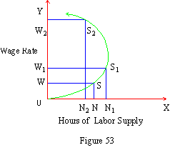Leisure is an attractive alternative to work and hence it is the opportunity cost at further hikes in the wage rate. This has been shown in Figure 53.

In the figure the number of hours of labor supplied have been measured along OX axis and the rate of wages along OY axis. When the initial wage rate is as low as W a worker supplies N hours of labor. With a rise in the rate of wages to W1 he has an incentive to work longer and to earn a higher income. Therefore the worker offers more hours of labor (N1). The labor supply curve SS1 slopes upwards as is normally expected. Beyond W1 if the wage rises further as W2 the worker may withdraw some hours of labor. He may prefer more leisure than work. Therefore supply of labor drops to fewer hours as N2. The supply curve S1S2 bends backward.

This is the typical nature of the labor supply curve. This can be explained both with the help of income and substitution effects. Beyond point S1 and wage rate W1 the worker feels that an adequate income has already been earned by him. Therefore beyond this point he prefers leisure to income. This is termed the negative income effect. Also, more work and more income, on the one hand, and more leisure, on the other, are substitutes of each other. About 10 or 12 hours of work leisure may be given up in preference to income but, beyond that, leisure is considered more valuable. Therefore it is substituted in place of work and income.

(B) Market Demand and Supply Curves for Labor: Under a perfect competitive market both demand and supply curves are likely to be normal in behavior. Demand curve for labor will then be downward sloping. In a market numerous firms operate; so the demand curve will be more flexible than in the case of individual firms. Labor supply curve will be composed of the additions of labor supplied by individuals. This is likely to slope upwards. It indicates that both labor of a higher quality and skills are supplied only at a rising rate of wages. Under competition, with a very large number of workers and with less significant personal differences, the supply curve will be highly flexible tending to be a horizontal straight line. Given the demand and supply schedules or curves competitive market equilibrium can be determined.

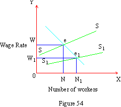
In Figure 54, DD and SS represent the competitive labor demand curve and the competitive supply curve respectively. The two curves intersect at point e which is a point of equilibrium. Under equilibrium condition, N number of workers offer supply of labor and receive the wage rate W. If labor market shows a greater homogeneity and if the qualitative variations are very few then the supply curve will be more flexible as represented by S1S1. With such a supply curve under the given demand conditions, a new point of equilibrium e1 is established. At this point more workers N1 offer services at a lower wage rate W1. Thus demand and supply conditions together determine level of employment and rate of wages in a competitive market.