14.4 Monopsony and Exploitation of Labor

(A) Monopsony: Monopoly in the product market is a condition where only one producer or seller operates. Similarly when only one employer is buying labor he enjoys monopsony power in the labor market. The workers have no option but to work with the monopsonist and to accept whatever wage rate is offered by him. The presence of monopsony causes a lower rate of wages than what the workers ordinarily deserve. Such a situation results in exploitation of labor. By exploitation, we mean that a smaller wage remuneration is paid to the workers than what they are entitled to receive under competitive rule. There are two possible cases of exploitation. In one case, monopoly power is enjoyed only in the labor market. In the other case, the producer is a monopolist both in the labor and the product markets.

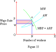
(B) Monopsony and Competition: A producer has monopsony power only in the labor market. In the product market he faces competition with other firms. In Figure 55 we notice such a situation.

In a competitive commodity market the demand curve of the producer is at once both the Marginal Revenue Product and the Average Revenue Product (MRP = ARP) curve. Because of uniform product price both values are identical. In the labor market, however, he has control over the labor supply. Therefore the supply curve slopes upwards. The value of Marginal Wage (MW) differs from Average Wage (AW). Both the MW and AW curves slope upward but MW is above AW. The firm is in equilibrium at point e with MRP = MW. In equilibrium position, N number of workers are employed and the price of the product is P. The total revenue of the firm is OPeN. The actual rate of wages paid is decided by the point of intersection L on the AW curve. The average wage of N workers is NL = OW. The total wage payment is of the size OWLN. The difference between the two areas is the value of exploitation of labor.

Exploitation = Total Revenue - Total wage cost = OPeN - OWLN = WPeL

(C) Monopsony and Monopoly: Besides being a monopsonist if the producer happens to be a monopolist in the product market as well then his surplus will be further enlarged.

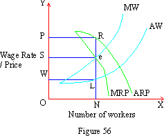
In Figure 56, we find that the producer enjoys monopoly power in both markets. Being a monopsonist in the labor market his MW - AW curves slope upwards as in the earlier case. Since he is a monopolist in the product market as well his marginal and average revenue product curves slope down and are distinct. MRP is below ARP. Once again the producer strikes equilibrium at point e where MRP = MW. At this point, N number of workers are employed. The price of the product is determined by a relevant point R on the AR curve. The price is NR = OP. At this price, total revenue of the firm is OPRN. Wage rate is determined by the value of the average wage. It is therefore NL = OW. At this wage rate, the total wage payment is OWLN. The difference between the areas is the no profit surplus of the producer.

Net Profit Surplus = OPRN - OWLN = WPRL

The entire surplus is split into two parts:

i) SPRe as surplus due to monopoly power in the producer market.

ii) WSeL as exploitation of labor due to monopsony power in the labor market.

The presence of monopsony has similar undesirable effects such as high price, low level of output, underutilization of capacity of production and loss of consumer surplus.