2.4 Elasticity of Demand and Supply

(A) Price Elasticity

i) Elasticity of Demand: Elasticity of demand can be classified into two major divisions: one the highly elastic, unitary elastic and the highly inelastic type and two, the extreme cases of the perfectly elastic and the perfectly inelastic type.

a) Highly elastic, Unitary elastic and highly inelastic: The laws of demand and supply are no doubt an important part of economic analysis. But the knowledge about demand and supply relations serves only a limited purpose. This is in view of the fact that both demand and supply laws are applicable to all kinds of goods. However, an actual rise or fall in the quantity demanded or supplied with a small variation in the price may considerably differ for different goods such as food, automobiles, film shows, garments, hardware materials, machines, land etc. In other words it is important to know the extent of rise or fall in the demand with a given change in the price for each individual good. This is exactly the purpose served by the concept of price elasticity of demand; this concept is advanced and subtle in nature. It was first developed by Alfred Marshall; he has defined elasticity as follows:

Elasticity of demand is the degree of responsiveness with which quantity demanded changes for a given change in price.

In other words it is a proportional change in the quantity demanded to a proportional change in price.

Price Elasticity of demand is then the ratio of the proportional change in the quantity demanded to the proportional change in price.

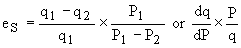
Proportional change in quantity can be expressed as        where q₁ is the initial and q₂ is the new quantity demanded.

Proportional change in price is similarly  &nbspwhere P₁ is initial and P₂ is the new price.

Elasticity ratio e is therefore,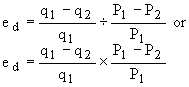    

If symbols q and P are used for small variations in quantity and price respectively then,

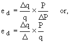
Note that Dq / Dp is in the limit derivative or marginal change and p/q is the reciprocal of average change, therefore

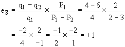
Let’s illustrate this. In our demand schedule example above, when price changes from 2 to 3 units, the quantity demanded changes from 4 to 1 units. Substituting these values we have:

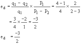
Note that the elasticity ratio 3/2 is more than one and has a negative sign. Both these are important features. Numerical values explain the extent or degree of change in demand while the sign of the ratio explains the direction of change. Since the law of demand is based on the inverse relation between price and quantity, the elasticity of demand is always stated with a negative sign.

The numerical value of elasticity can be equal to 1 (that is called ‘unit’) more than one or less than one. In case of unit elastic demand (e = 1) both price and quantity (demanded) changes occur in the same proportion. If the value of elasticity exceeds one (e > 1) then the percentage or proportional change in quantity demanded is greater than that in price and the good is said to be price elastic or highly responsive to a change in price. If the value of elasticity is less than one (e < 1) then the proportional change in quantity is smaller than that in price and the demand for the good is said to be price inelastic or not very responsive to a change in price. The information about the value of elasticity therefore serves an important purpose in classification of various goods as elastic or inelastic in demand. This helps in several practical and policy applications such as taxation, foreign trade, monopoly, price determination etc.

There are four methods of measurement of elasticity of demand. These are percentage, proportion, outlay and geometric or point elasticity methods. The one mentioned last (point elasticity method) is the most accurate and can be explained conveniently with a given demand curve:



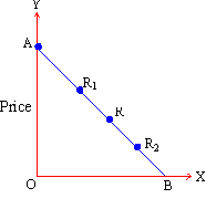
Quanti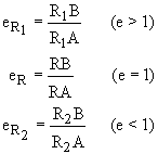ty demanded

Figure 6

In the figure, AB is the demand curve and at any point on this, the elasticity of demand can be measured. At points R₁, R and R₂ the values of elasticity are:

At the mid point R on the demand curve, the value of elasticity is unit or equal to one. But above point R such as at R₁, the value of elasticity is more than one and demand is highly elastic. On the other hand at a lower point such as R₂ demand becomes inelastic as the value of elasticity is less than one. In general as we move in the direction of the Y axis, demand becomes more and more elastic. But as we move in the direction of the X axis, demand becomes less and less elastic. In other words at every higher price demand is relatively more elastic and at every lower price demand is relatively less elastic. This also explains that elasticity of demand differs not only from commodity to commodity but also for the same commodity at varying prices.

b) Two extreme cases: Besides the three explained above, two more extreme values of price elasticity of demand can be included in the analysis. These are:

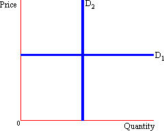
(i) Perfectly Price Elastic: At this extreme, for any small decrease in price, the increase in the quantity demanded is infinitely large. In such a case, demanders demand all the can. Here the demand is said to be perfectly price elastic (e = that is infinity). This is represented graphically as a horizontal demand curve (D₁ in the figure above).

(ii) Perfectly Price Inelastic: At this extreme, for any change in price there is no change in the quantity demanded. Therefore the demand is completely unresponsive to any change in price. In this case the demand is said to be perfectly price inelastic (e = 0). This is represented graphically by a vertical demand curve (D₂ in the figure above).

ii) Elasticity of Supply: Like demand, elasticity of supply can also be classified into two major divisions: one the highly elastic, unitary elastic and highly inelastic type and two, the extreme cases of the perfectly elastic and the perfectly inelastic type.

a) Highly elastic, unitary elastic and highly inelastic: Elasticity of supply can similarly be defined and computed at varying prices and quantities supplied.

Elasticity of supply is the degree of responsiveness with which quantity supplied changes with a given change in the price.

This can be expressed with a similar formula:

An important difference between the price elasticity of demand and that of supply is that the latter is positive in value (as against the negative value in case of elasticity of demand). This is obvious from the fact that supply is a direct function of price: and both quantity and price change in the same direction. This will be clear from the following example. The values of ‘q’ and ‘P’ have been selected from the supply schedule given above.

The elasticity of supply also shows variations in its value for different commodities. Accordingly supply elasticity for different goods can be unit, (e_s = 1) more than one (e_s > 1) or less than one (e_s < 1). The goods can then be categorized as relatively elastic or inelastic in supply. Elasticity of supply is also of considerable practical importance in its policy applications.

b) Two extreme cases: Besides the three explained above, two extreme values of price elasticity of supply can be included in the analysis:

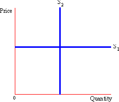
i) Perfectly Price Elastic: At this extreme for any small decrease in price, the quantity supplied is infinitely large. In such a case, suppliers supply all they can. Here the supply is said to be perfectly price elastic (e = that is infinity). This is represented graphically by a horizontal supply curve (S₁ in the figure below).

ii) Perfectly Price Inelastic: At this extreme for any change in price there is no change in the quantity supplied. Therefore the supply is completely indifferent to any change in price (e = 0). Here the supply is said to be perfectly price inelastic. This is represented graphically by a vertical supply curve (S₂ in the figure below).

Figure 8